Skip to content

Every driver in this package returns the same kind of object, a nested_results, and the getting-started guide, vignette("nested-cv"), reads three things off it: the print, the summary and the estimate. This page reads the whole object. It walks the columns one at a time, runs each of the readers on one result, shows what a run looks like when one outer fold fails, says which dplyr verbs keep the class and which shed it, and ends with the two arguments the runs above do not use, event_level and eval_time.

The run

The design, the workflow and the grid are the guide’s, unchanged: five outer folds of mtcars, five inner folds under each, and a random forest with two parameters marked for tuning.

set.seed(1)

folds <- nested_resamples(
  mtcars,
  outside = vfold_cv(v = 5),
  inside = vfold_cv(v = 5)
)

rf <- rand_forest(mtry = tune(), min_n = tune(), trees = 500) |>
  set_engine("ranger") |>
  set_mode("regression")

wf <- workflow(mpg ~ ., rf)

grid <- expand.grid(mtry = c(2L, 5L, 8L), min_n = c(2L, 10L))
set.seed(2)

res <- nested_tune_grid(wf, folds, grid = grid)

res
#> 
#> ── Nested cross-validation results ────────────────────────────────────
#> Outer resamples: 5-fold cross-validation
#> # A tibble: 5 × 9
#>   splits         id    .metrics .selected .inner_metrics    .notes  
#>   <list>         <chr> <list>   <list>    <list>            <list>  
#> 1 <split [25/7]> Fold1 <tibble> <tibble>  <tibble [12 × 8]> <tibble>
#> 2 <split [25/7]> Fold2 <tibble> <tibble>  <tibble [12 × 8]> <tibble>
#> 3 <split [26/6]> Fold3 <tibble> <tibble>  <tibble [12 × 8]> <tibble>
#> 4 <split [26/6]> Fold4 <tibble> <tibble>  <tibble [12 × 8]> <tibble>
#> 5 <split [26/6]> Fold5 <tibble> <tibble>  <tibble [12 × 8]> <tibble>
#> # ℹ 3 more variables: .completed <lgl>, .tuning_seed <int>,
#> #   .outer_fit_seed <int>
#>  Use `summary()` for what the run means: which folds failed, what
#>   each one selected, and the estimate across them.

What the columns hold

The object is a tibble with one row per outer fold, and the print above shows its columns. Each holds one piece of what that fold did.

names(res)
#> [1] "splits"          "id"              ".metrics"       
#> [4] ".selected"       ".inner_metrics"  ".notes"         
#> [7] ".completed"      ".tuning_seed"    ".outer_fit_seed"

splits is the fold’s outer split, an ordinary rsample split whose analysis rows the tuning saw and whose assessment rows scored the fold’s model.

res$splits[[1]]
#> <Analysis/Assess/Total>
#> <25/7/32>

id is the fold’s label, copied from the design. A repeated design carries more than one label column, and the object records which columns they are.

res$id
#> [1] "Fold1" "Fold2" "Fold3" "Fold4" "Fold5"

.metrics is the score of the fold’s finalized model on its assessment rows, one row per metric, in the shape tune::last_fit() produces. It is what collect_metrics() averages.

res$.metrics[[1]]
#> # A tibble: 2 × 4
#>   .metric .estimator .estimate .config        
#>   <chr>   <chr>          <dbl> <chr>          
#> 1 rmse    standard       1.23  pre0_mod0_post0
#> 2 rsq     standard       0.911 pre0_mod0_post0

.selected is the candidate the fold’s inner tuning chose, a one-row tibble of the tuned parameters. It is what summary(), agreement() and the default autoplot() read.

res$.selected[[1]]
#> # A tibble: 1 × 3
#>    mtry min_n .config        
#>   <int> <int> <chr>          
#> 1     8     2 pre0_mod5_post0

.inner_metrics is the whole table the inner search scored, every candidate on every inner resample, averaged. It is what the fold’s selection was made from, and vignette("tuners") shows how its shape differs by search.

res$.inner_metrics[[1]]
#> # A tibble: 12 × 8
#>     mtry min_n .metric .estimator  mean     n std_err .config        
#>    <int> <int> <chr>   <chr>      <dbl> <int>   <dbl> <chr>          
#>  1     2     2 rmse    standard   2.87      5  0.435  pre0_mod1_post0
#>  2     2     2 rsq     standard   0.814     5  0.0935 pre0_mod1_post0
#>  3     2    10 rmse    standard   3.09      5  0.548  pre0_mod2_post0
#>  4     2    10 rsq     standard   0.776     5  0.115  pre0_mod2_post0
#>  5     5     2 rmse    standard   2.88      5  0.446  pre0_mod3_post0
#>  6     5     2 rsq     standard   0.834     5  0.0900 pre0_mod3_post0
#>  7     5    10 rmse    standard   2.88      5  0.510  pre0_mod4_post0
#>  8     5    10 rsq     standard   0.803     5  0.115  pre0_mod4_post0
#>  9     8     2 rmse    standard   2.85      5  0.419  pre0_mod5_post0
#> 10     8     2 rsq     standard   0.834     5  0.0942 pre0_mod5_post0
#> 11     8    10 rmse    standard   2.89      5  0.497  pre0_mod6_post0
#> 12     8    10 rsq     standard   0.805     5  0.115  pre0_mod6_post0

.notes holds what went wrong inside the fold, in tune’s shape with a location naming the stage. A fold that ran cleanly has no rows.

res$.notes[[1]]
#> # A tibble: 0 × 4
#> # ℹ 4 variables: location <chr>, type <chr>, note <chr>, trace <list>

.completed says whether the fold produced a score. The section on a failed fold below shows a FALSE.

res$.completed
#> [1] TRUE TRUE TRUE TRUE TRUE

.tuning_seed and .outer_fit_seed are the two seeds each fold ran under, drawn at entry and fixed by the fold’s position in the design. The guide’s reproducibility section shows how to restore them, and the help pages for nested_tune_grid() and nested_final_fit() give the recipe for replaying one fold by hand.

res[, c(".tuning_seed", ".outer_fit_seed")]
#> # A tibble: 5 × 2
#>   .tuning_seed .outer_fit_seed
#>          <int>           <int>
#> 1    794080207       314911494
#> 2   1906307464       554751325
#> 3   2010156236       226245929
#> 4   1118907979      1740692099
#> 5   2046114256      1910444850

The description of the run itself rides on the object as attributes rather than columns, and vignette("tuners") reads one of them, procedure.

The readers

Printing describes the object in hand. summary() says what the run means: how much of the design ran, what each fold chose, and the estimate.

summary(res)
#> 
#> ── Nested cross-validation results ────────────────────────────────────
#> Outer resamples: 5-fold cross-validation
#> Outer folds: 5 requested, 5 completed
#> 
#> ── Selected parameters ──
#> 
#> ! mtry: 8, 8, 5, 8, 5 (folds disagree)
#>  min_n: 2 (all 5 completed folds agree)
#> 
#> ── Estimate (5 of 5 outer folds) ──
#> 
#> rmse (standard): 2.49
#> rsq (standard): 0.842
#> 
#>  A nested estimate describes the tune-and-fit procedure, not a model
#>   you can deploy. Build that with `nested_final_fit()`, and report
#>   this estimate as what its procedure achieves.

collect_metrics() is the estimate as a table, the mean and standard error of the outer scores. With summarize = FALSE it is the outer scores themselves, one row per fold and metric, which is each fold’s .metrics rows, less .config, with the fold label beside them.

collect_metrics(res)
#> # A tibble: 2 × 5
#>   .metric .estimator  mean     n std_err
#>   <chr>   <chr>      <dbl> <int>   <dbl>
#> 1 rmse    standard   2.49      5  0.447 
#> 2 rsq     standard   0.842     5  0.0293

collect_metrics(res, summarize = FALSE)
#> # A tibble: 10 × 4
#>    id    .metric .estimator .estimate
#>    <chr> <chr>   <chr>          <dbl>
#>  1 Fold1 rmse    standard       1.23 
#>  2 Fold1 rsq     standard       0.911
#>  3 Fold2 rmse    standard       3.22 
#>  4 Fold2 rsq     standard       0.819
#>  5 Fold3 rmse    standard       2.48 
#>  6 Fold3 rsq     standard       0.805
#>  7 Fold4 rmse    standard       1.83 
#>  8 Fold4 rsq     standard       0.766
#>  9 Fold5 rmse    standard       3.69 
#> 10 Fold5 rsq     standard       0.911

agreement() counts the selections: one row per distinct combination the folds chose, with how many completed folds chose it, n, and that count as a share of the completed folds, prop. The most frequent row describes how stable the tuning procedure’s choice was on this data. It is not the final model’s parameters, which come from nested_final_fit() running the procedure once more on the whole dataset.

agreement(res)
#> # A tibble: 2 × 4
#>    mtry min_n     n  prop
#>   <int> <int> <int> <dbl>
#> 1     8     2     3   0.6
#> 2     5     2     2   0.4

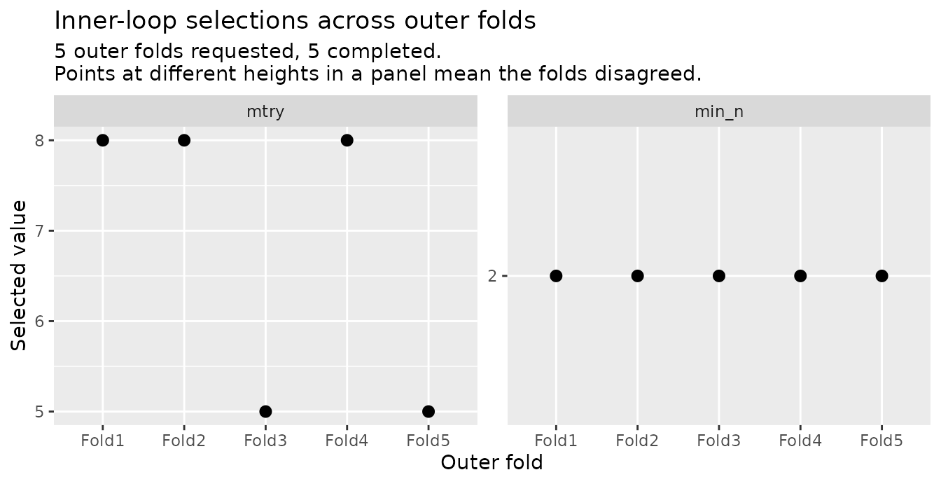
autoplot() draws the same two facts. The default view is the selections, one panel per tuned parameter and one point per outer fold.

One panel per tuned parameter, mtry and min_n, with one point per outer fold at the value that fold's inner tuning selected.

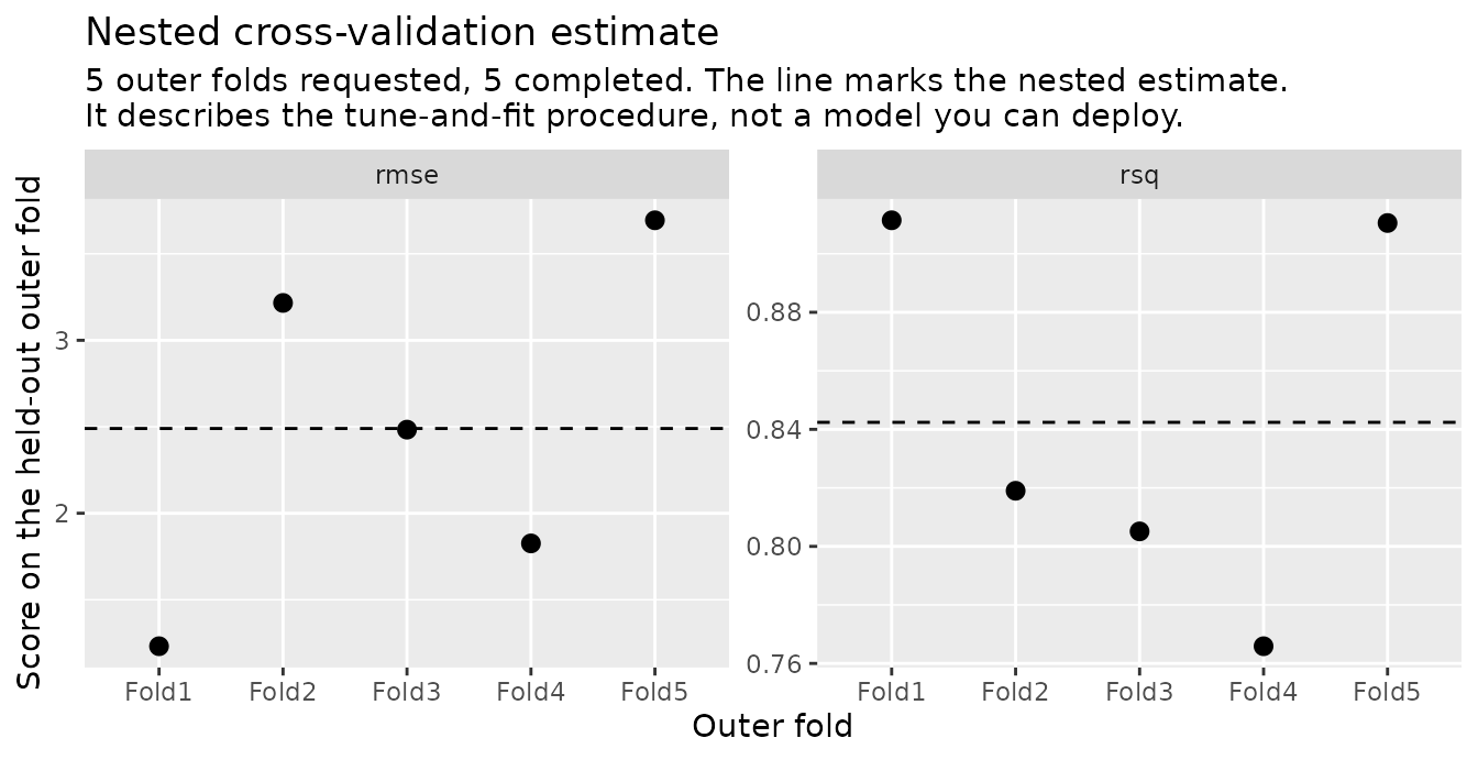
The other view is the outer scores, one panel per metric and one point per fold, with a dashed line at the mean that collect_metrics() reports.

autoplot(res, type = "performance")

One panel per metric, rmse and rsq, with one point per outer fold's score on its assessment rows and a dashed line at the mean across folds.

When a fold fails

A fold that fails does not end the run. The other folds keep their results, and the fold that failed is recorded rather than dropped. To show that on the guide’s run, the workflow below adds one preprocessing step a careful reader might write anyway: a range check on horsepower, which refuses to predict for a car whose horsepower lies outside the range the model was trained on, beyond a small slack. One car, the Maserati Bora, has far more horsepower than any other in mtcars, 335 against 264 for the next. The fold that holds it out cannot score it, and that fold fails.

library(recipes)

rec <- recipe(mpg ~ ., data = mtcars) |>
  check_range(hp)

wf_checked <- workflow(rec, rf)
set.seed(2)

failed <- nested_tune_grid(wf_checked, folds, grid = grid)
#> Warning: All models failed. Run `show_notes(.Last.tune.result)` for more
#> information.
#> Warning in nested_tune_grid(wf_checked, folds, grid = grid): ! 1 of 5 outer folds failed.
#>  Failed: "Fold1".
#>  See `x$.notes` for what went wrong.

stopifnot(sum(!failed$.completed) == 1L)
failed
#> 
#> ── Nested cross-validation results ────────────────────────────────────
#> Outer resamples: 5-fold cross-validation
#> # A tibble: 5 × 9
#>   splits         id    .metrics .selected .inner_metrics    .notes  
#>   <list>         <chr> <list>   <list>    <list>            <list>  
#> 1 <split [25/7]> Fold1 <tibble> <NULL>    <tibble [12 × 8]> <tibble>
#> 2 <split [25/7]> Fold2 <tibble> <tibble>  <tibble [12 × 8]> <tibble>
#> 3 <split [26/6]> Fold3 <tibble> <tibble>  <tibble [12 × 8]> <tibble>
#> 4 <split [26/6]> Fold4 <tibble> <tibble>  <tibble [12 × 8]> <tibble>
#> 5 <split [26/6]> Fold5 <tibble> <tibble>  <tibble [12 × 8]> <tibble>
#> # ℹ 3 more variables: .completed <lgl>, .tuning_seed <int>,
#> #   .outer_fit_seed <int>
#>  1 of 5 outer folds did not complete.
#>  Use `summary()` for what the run means: which folds failed, what
#>   each one selected, and the estimate across them.

The run warns twice as it finishes: tune’s own warning from the outer fit that produced nothing, then this package’s, naming the fold. The chunk mutes tune’s progress messages and keeps its warnings. The print counts the failure, .completed is FALSE for the fold that failed, and its .notes say where.

which_failed <- which(!failed$.completed)

failed$.notes[[which_failed]][, c("location", "type", "note")]
#> # A tibble: 2 × 3
#>   location                                      type  note             
#>   <chr>                                         <chr> <chr>            
#> 1 outer fit                                     error "The outer fit p…
#> 2 outer fit: preprocessor 1/1 (prediction data) error "\u001b[1m\u001b…

The first row is this package’s own note, and its location names the stage: Fold1 failed at the outer fit, the fit and score on the outer split, after its inner tuning had finished. The rows after it are tune’s notes about the cause, relabelled with the stage they came from. A fold that fails during inner tuning reads the same way with inner tuning as the stage.

A fold can also complete and carry notes. The Maserati sits in the analysis set of every other fold, so each of those folds had one inner resample that held it out, and the range check refused that resample for every candidate. Some folds carry a second note of the same kind from the low end of the range, an inner resample that held out a car with less horsepower than any it trained on. Tuning still returned a candidate, from the inner resamples that ran, and the fold finished. Its notes say so.

vapply(failed$.notes, nrow, integer(1))
#> [1] 2 2 1 1 1

noted <- which(failed$.completed & vapply(failed$.notes, nrow, integer(1)) > 0)

failed$id[noted[1]]
#> [1] "Fold2"

failed$.notes[[noted[1]]][, c("location", "type", "note")]
#> # A tibble: 2 × 3
#>   location                                                 type  note  
#>   <chr>                                                    <chr> <chr> 
#> 1 inner tuning (Fold3): preprocessor 1/1 (prediction data) error "\u00…
#> 2 inner tuning (Fold5): preprocessor 1/1 (prediction data) error "\u00…

The label in parentheses names the inner resample, a fold of this outer fold’s own inner design, not another outer fold. So .completed being TRUE beside a non-empty .notes means exactly this: the fold worked, on less than the whole inner design it was given.

summary() on a run with a failed fold still answers, and warns first. The chunk below catches the warning to show its class and its message, then prints the summary it returned.

partial <- withCallingHandlers(
  summary(failed),
  warning = function(w) {
    cat("class:", class(w)[1], "\n")
    cat(conditionMessage(w), "\n")
    invokeRestart("muffleWarning")
  }
)
#> class: nestedtune_partial_summary 
#> ! This summary covers 4 of 5 outer folds.
#>  Failed: "Fold1".
#>  It describes the folds that ran, not the design that was requested.

partial
#> 
#> ── Nested cross-validation results ────────────────────────────────────
#> Outer resamples: 5-fold cross-validation
#> Outer folds: 5 requested, 4 completed
#>  Fold1 failed during outer fit.
#>  See the `.notes` column of the results object for what went wrong.
#> 
#> ── Selected parameters ──
#> 
#> ! mtry: 8, 5, 8, 2 (folds disagree)
#> ! min_n: 10, 2, 2, 2 (folds disagree)
#> 
#> ── Estimate (4 of 5 outer folds) ──
#> 
#> rmse (standard): 2.95
#> rsq (standard): 0.814
#> 
#>  A nested estimate describes the tune-and-fit procedure, not a model
#>   you can deploy. Build that with `nested_final_fit()`, and report
#>   this estimate as what its procedure achieves.

The warning’s class lets a script catch it and decide what a partial run is worth. The message names how many folds the summary covers and how many the design asked for, and the summary itself describes the folds that ran: the selections are those 4 folds’ selections, and the estimate is the mean over their 4 scores, with the failed fold absent rather than filled in. collect_metrics() and agreement() warn the same way, and autoplot() leaves the failed fold’s place on its axis empty. A run in which no fold completed is different: summary() still describes it, but collect_metrics(), agreement(), autoplot() and nested_final_fit() refuse it, because there is no estimate to report for a design that did not execute.

What dplyr keeps and what it sheds

The object is a tibble, so dplyr’s verbs work on it, and one rule decides what they hand back: a verb that only reorders the rows or adds or reorders columns returns a nested_results, and a verb that adds or removes a row, or drops or overwrites one of the columns above, returns a bare tibble, because an object that no longer holds what the run produced cannot answer for the run. Adding a column keeps the class.

with_rmse <- dplyr::mutate(
  res,
  rmse = vapply(.metrics, function(m) m$.estimate[m$.metric == "rmse"], 1)
)

class(with_rmse)
#> [1] "nested_results" "tbl_df"         "tbl"            "data.frame"

Dropping a fold sheds it. The natural case is keeping only the folds that completed on the run above, which removes one row.

completed_only <- dplyr::filter(failed, .completed)

class(completed_only)
#> [1] "tbl_df"     "tbl"        "data.frame"

So does a column subset that leaves the run’s record behind, through base [ rather than a dplyr verb, since the same rule governs it.

class(res[, "id"])
#> [1] "tbl_df"     "tbl"        "data.frame"

Both of those hand back the data and nothing more: a plain tibble print, no summary of the run, no collect_metrics(). That is the point. A four-row table cannot describe itself as a five-fold design, so it stops describing itself. To read a partial run, read the run: collect_metrics(failed) already averages the folds that completed, and warns that it did.

Two more arguments: event_level and eval_time

Every tuning driver takes two more arguments than the runs above used, and both reach tune untouched; nested_final_fit() reads them back from the results object instead. event_level is for classification: it names which level of the outcome factor counts as the event, "first" unless you say otherwise, and it sets the same slot on the inner tuning and on the outer scoring fit at once. A regression or censored-regression run ignores it, as tune does. eval_time is for censored regression, and it changes the shape of the result, so the rest of this section runs one.

set.seed(51)

n <- 180
x1 <- rnorm(n)
x2 <- rnorm(n)
lp <- 0.9 * x1 - 0.6 * x2
early <- rbinom(n, 1, 0.45)
event_time <- ifelse(
  early == 1,
  runif(n, 0.02, 0.6) * exp(-lp / 6),
  rlnorm(n, meanlog = log(15) - lp, sdlog = 0.8)
)
censor_time <- runif(n, 3, 60)

surv_df <- data.frame(
  time = pmin(event_time, censor_time),
  event = as.numeric(event_time <= censor_time),
  x1 = x1,
  x2 = x2
)

The data is simulated: two predictors, a time, and an event indicator that is zero where the observation was censored before its event. The model is a parametric survival regression whose one tunable is the distribution of the event times, and the grid names three.

library(censored)

surv_spec <- survival_reg(dist = tune()) |>
  set_engine("survival") |>
  set_mode("censored regression")

surv_wf <- workflow(survival::Surv(time, event) ~ x1 + x2, surv_spec)

surv_grid <- data.frame(dist = c("weibull", "lognormal", "exponential"))

A dynamic survival metric is evaluated at a time: the Brier score at one time asks how well the model predicts who has survived to that point. So the metric has one value per time, and eval_time is where the times are given. They reach the inner tuning, which selects on the first of them and warns once per fold to say so (the chunk mutes those warnings), and the outer scoring fit, which scores at each.

set.seed(61)

surv_folds <- nested_resamples(
  surv_df,
  outside = vfold_cv(v = 3),
  inside = vfold_cv(v = 3)
)

set.seed(62)

surv_res <- nested_tune_grid(
  surv_wf,
  surv_folds,
  grid = surv_grid,
  metrics = yardstick::metric_set(yardstick::brier_survival),
  eval_time = c(0.5, 10)
)

collect_metrics(surv_res)
#> # A tibble: 2 × 6
#>   .metric        .estimator .eval_time  mean     n std_err
#>   <chr>          <chr>           <dbl> <dbl> <int>   <dbl>
#> 1 brier_survival standard          0.5 0.251     3 0.00584
#> 2 brier_survival standard         10   0.222     3 0.00901

The estimate carries an .eval_time column, and has one row per metric and time: the Brier score at 0.5 and at 10, each the mean over the outer folds of that fold’s score at that time. The per-fold table carries the same column, and so does each fold’s .metrics.

collect_metrics(surv_res, summarize = FALSE)
#> # A tibble: 6 × 5
#>   id    .metric        .estimator .eval_time .estimate
#>   <chr> <chr>          <chr>           <dbl>     <dbl>
#> 1 Fold1 brier_survival standard          0.5     0.259
#> 2 Fold1 brier_survival standard         10       0.230
#> 3 Fold2 brier_survival standard          0.5     0.240
#> 4 Fold2 brier_survival standard         10       0.204
#> 5 Fold3 brier_survival standard          0.5     0.255
#> 6 Fold3 brier_survival standard         10       0.231

surv_res$.selected[[1]]
#> # A tibble: 1 × 2
#>   dist      .config        
#>   <chr>     <chr>          
#> 1 lognormal pre0_mod2_post0

Everything else reads as before. agreement() counts the selected distributions the way it counted mtry above:

agreement(surv_res)
#> # A tibble: 2 × 3
#>   dist          n  prop
#>   <chr>     <int> <dbl>
#> 1 lognormal     2 0.667
#> 2 weibull       1 0.333

summary() and the default autoplot() read the same .selected column, and autoplot(type = "performance") draws one panel per metric and time.